DP 10-2
Discovery Project ■ Computer Graphics III
Objective Learn how to rotate an image using rotation matrices.
In the Discovery Project Computer Graphics I we saw how matrix multiplication is used in computer graphics. We found matrices that reflect, expand, or shear an image. We now consider matrices that rotate an image, as in the graphics shown here.
Rotating Points in the Plane
Recall that a point $(x, y)$ in the plane is represented by the $2 \times 1$ matrix $\left[ \begin{array}{} x\\ y \end{array} \right]$. The matrix that rotates this point about the origin through an angle $ ɸ$ is $$R = \left[ \begin{array}{} \cos \; ɸ-\sin \; ɸ\\ \sin \; ɸ \;\;\; \cos \; ɸ \end{array} \right] \quad \color{#08F}{\textrm{Rotation} \; \textrm{matrix}}$$
Note that rotating a point counter-clockwise corresponds to rotating the axes clockwise.
When the point $P = \left[ \begin{array}{} x\\ y \end{array} \right]$ is rotated clockwise about the origin through an angle $ɸ$, it moves to a new location $P' = \left[ \begin{array}{} x'\\ y' \end{array} \right]$ given by the matrix product $P' = RP$, as shown in Figure 1.
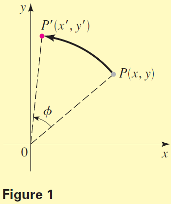
$$P' = RP = \left[ \begin{array}{} \cos \; ɸ-\sin \; ɸ\\ \sin \;ɸ \;\;\; \cos \; ɸ \end{array} \right] \left[ \begin{array}{} x\\ y \end{array} \right] = \left[ \begin{array}{} x \; \cos \; ɸ - y \; \sin \; ɸ\\ x \; \sin \; ɸ + y \; \cos \; ɸ \end{array} \right]$$
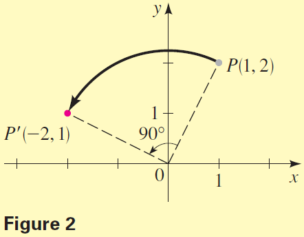
For example, if $ɸ = 90^\circ$, the rotation matrix is $$R = \left[ \begin{array}{} \cos \; 90^\circ &-\sin \; 90^\circ\\ \sin \; 90^\circ & \;\;\; \cos \; 90^\circ \end{array} \right] = \left[ \begin{array}{} 0&-1 \\ 1& \;\;\; 0 \end{array} \right] \quad \color{#08F}{\textrm{Rotation} \; \textrm{matrix} \; (ɸ = 90^\circ)}$$
Applying a $90^\circ$ rotation to the point $P = \left[ \begin{array}{} 1 \\ 2 \end{array} \right]$ moves it to the point $$P' = RP = \left[ \begin{array}{} 0&-1 \\ 1& \;\;\; 0 \end{array} \right]\left[ \begin{array}{} 1 \\ 2 \end{array} \right] = \left[ \begin{array}{} -2 \\ \;\;\; 1 \end{array} \right]$$
See Figure 2.
Rotating Images in the Plane
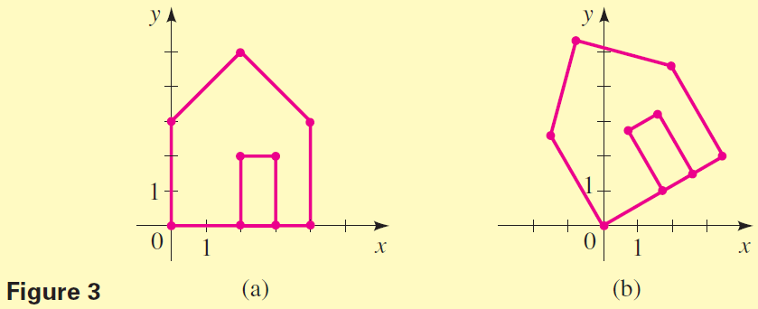
If the rotation matrix is applied to every point in an image, then the entire image is rotated. To rotate the house in Figure 3(a) through a $30^\circ$ angle about the origin, we multiply its data matrix by the rotation matrix that has $ɸ = 30^\circ$.
$$RD = \left[ \begin{array}{} \frac{\sqrt 3}{2} & -\frac 12 \\ \frac 12 & \frac{\sqrt 3}{2} \end{array} \right] \left[ \begin{array}{} 2&0&0&2&4&4&3&3&2&2&3 \\ 0&0&3&5&3&0&0&2&2&0&0 \end{array} \right]$$ $$ \qquad \qquad \qquad \qquad \qquad \quad \approx \left[ \begin{array}{} 1.73&0&-1.50&-0.77&1.96&3.46&2.60&1.60&0.73&1.73&2.60 \\ \;\; 1&0& \;\;\; 2.60& \;\;\; 5.33&4.60& \;\; 2&1.50&3.23&2.73& \;\; 1&1.50 \end{array} \right]$$The new data matrix $RD$ represents the rotated house in Figure 3(b).
The Discovery Project: Computer Graphics II describes a TI-83 program that draws the image corresponding to a given data matrix. You may find it convenient to use this program in some of the following activities.
Problems
- Use a rotation matrix to find the new coordinates of the given point when it is rotated through the given angle.
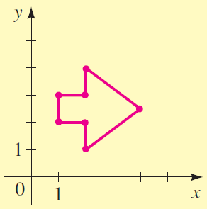
(a) $(1, 4), \; ɸ = 90^\circ$ (b) $(-2, 1), \; ɸ = 60^\circ$ (c) $(-2, -2), \; ɸ = 135^\circ$ (d) $(7, 3), \; ɸ = -60^\circ$ - Find a data matrix for the line drawing in the figure shown in the margin. Multiply the data matrix by a suitable rotation matrix to rotate the image about the origin by $ɸ = 120^\circ$. Sketch the rotated image given by the new data matrix.
- Sketch the image represented by the data matrix $D$. $$D = \left[
\begin{array}{}
2&3&3&4&4&1&1&2&2 \\
1&1&3&3&4&4&3&3&1
\end{array}
\right]$$
Find the rotation matrix $R$ that corresponds to a $45^\circ$ rotation, and the transformation matrix $T$ that corresponds to an expansion by a factor of $2$ in the $x$-direction. How does multiplying the data matrix by $RT$ change the image? How about multiplying by $TR$? Calculate the products $RTD$ and $TRD$, and sketch the corresponding images to confirm your answers.
- Let $R$ be the rotation matrix for the angle $ɸ$. Show that $R^{-1}$ is the rotation matrix for the angle $- ɸ$.
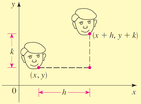
- To translate an image by $(h, k)$, we add $h$ to each $x$-coordinate and $k$ to each $y$-coordinate of each point in the image (see the figure in the margin). This can be done by adding an appropriate matrix $M$ to $D$, but the dimension of $M$ would change depending on the dimension of $D$. In practice, translation is accomplished by matrix multiplication. To see how this is done, we introduce homogeneous coordinates; that is, we represent the point $(x, y)$ by a $3 \times 1$ matrix:
$$(x, y) \leftrightarrow \left[ \begin{array}{cc|c} x \\ y \\ 1 \end{array} \right]$$
- Let $T$ be the matrix $$T = \left[
\begin{array}{}
1&0&h \\
0&1&k \\
0&0&1
\end{array}
\right]$$
Show that $T$ translates the point $(x, y)$ to the point $(x + h, y + h)$ by verifying the following matrix multiplication.$$\left[ \begin{array}{} 1&0&h \\ 0&1&k \\ 0&0&1 \end{array} \right]\left[ \begin{array}{} x \\ y \\ 1 \end{array} \right] = \left[ \begin{array}{} x + h \\ y + k \\ \;\;\; 1 \end{array} \right]$$
- Find $T^{-1}$ and describe how $T^{-1}$ translates points.
- Verify that multiplying by the following matrices has the indicated effects on a point $(x, y)$ represented by its homogeneous coordinates $\left[
\begin{array}{}
x \\
y \\
1
\end{array}
\right].$
$$(i)\left[
\begin{array}{}
1& \; 0&0 \\
0&-1&0 \\
0& \; 0&1
\end{array}
\right]\;\;\;\;(ii)\left[
\begin{array}{}
c&0&0 \\
0&1&0 \\
0&0&1
\end{array}
\right]\;\;\;\;(iii)\left[
\begin{array}{}
1&c&0 \\
0&1&0 \\
0&0&1
\end{array}
\right]\;\;\;\;(iv)\left[
\begin{array}{}
\cos \; ɸ-\sin \; ɸ &0 \\
\sin \; ɸ \;\;\; \cos \; ɸ &0 \\
\;\;\;0\;\;\;\;\;\;\;\;\;0&1
\end{array}
\right]$$
Reflection
$\;$in $x$-axisExpansion (or
$\;$ contraction)
$\;$in $x$-direction$\;$Shear in
$x$-directionRotation about the
$\qquad$origin by
$\; \quad$the angle $ɸ$
- Sketch the image represented (in homogeneous coordinates) by this data matrix: $$D = \left[
\begin{array}{}
3&5&5&7&7&9&9&7&7&5&5&3&3 \\
7&7&5&5&7&7&9&9&11&11&9&9&7 \\
1&1&1&1&1&1&1&1&1&1&1&1&1
\end{array}
\right] $$
Find a matrix $T$ that translates the image by $(-6, -8)$ and a matrix $R$ that rotates the image by $45^\circ$. Sketch the images represented by the data matrices $TD$, $RTD$, and $T^{-1}RTD$. Describe how an image is changed when its data matrix is multiplied by $T$, by $RT$, and by $T^{-1}RT$.
- Let $T$ be the matrix $$T = \left[
\begin{array}{}
1&0&h \\
0&1&k \\
0&0&1
\end{array}
\right]$$