DISCOVERY PROJECT
Iteration and Chaos
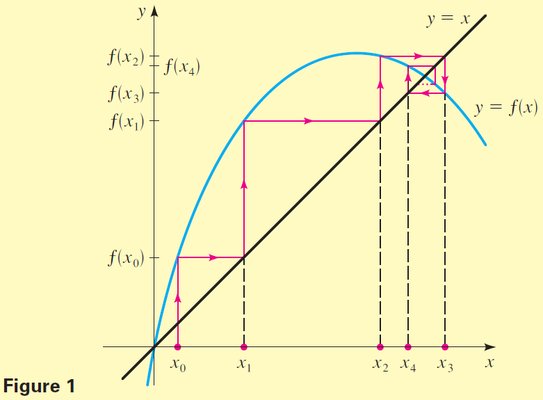
The iterates of a function $f$ at a point $x_0$ are $f(x_0)$, $f(f(x_0))$, $f(f(f(x_0)))$, and so on. We write
| $x_1 = f(x_0)$ | $\color{#08F}{The \; first \; iterate}$ | |
| $x_2 = f(f(x_0))$ | $\color{#08F}{The \; second \; iterate}$ | |
| $x_3 = f(f(f(x_0)))$ | $\color{#08F}{The \; third \; iterate}$ |
For example, if $f(x) = x^2$, then the iterates of $f$ at $2$ are $x_1 = 4$, $x_2 = 16$, $x_3 = 256$, and so on. (Check this.) Iterates can be described graphically as in Figure 1. Start with $x_0$ on the $x$-axis, move vertically to the graph of $f$, then horizontally to the line $y = x$, then vertically to the graph of $f$, and so on. The $x$-coordinates of the points on the graph of $f$ are the iterates of $f$ at $x_0$.
Iterates are important in studying the logistic function
$$f(x) = kx(1 - x)$$
| $n$ | $x_n$ |
|---|---|
| $\;$0 | $0.1$ |
| $\;$1 | $0.234$ |
| $\;$2 | $0.46603$ |
| $\;$3 | $0.64700$ |
| $\;$4 | $0.59382$ |
| $\;$5 | $0.62712$ |
| $\;$6 | $0.60799$ |
| $\;$7 | $0.61968$ |
| $\;$8 | $0.61276$ |
| $\;$9 | $0.61694$ |
| 10 | $0.61444$ |
| 11 | $0.61595$ |
| 12 | $0.61505$ |
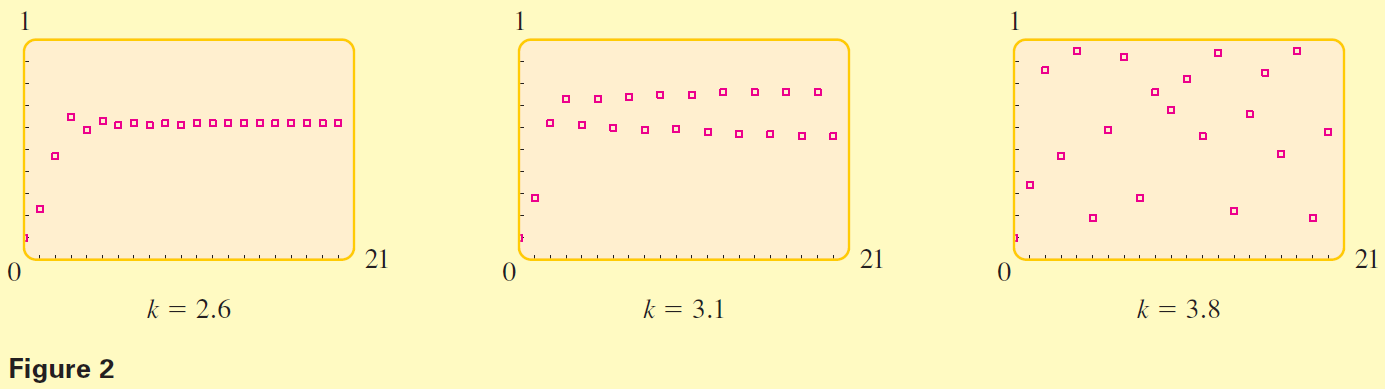
which models the population of a species with limited potential for growth (such as rabbits on an island or fish in a pond). In this model the maximum population that the environment can support is $1$ (that is, $100$%). If we start with a fraction of that population, say $0.1$ ($10$%), then the iterates of $f$ at $0.1$ give the population after each time interval (days, months, or years, depending on the species). The constant $k$ depends on the rate of growth of the species being modeled; it is called the growth constant. For example, for $k = 2.6$ and $x_0 = 0.1$ the iterates shown in the table to the left give the population of the species for the first $12$ time intervals. The population seems to be stabilizing around $0.615$ (that is, $61.5$% of maximum).
In the three graphs in Figure 2, we plot the iterates of $f$ at $0.1$ for different values of the growth constant $k$. For $k = 2.6$ the population appears to stabilize at a value $0.615$ of maximum, for $k = 3.1$ the population appears to oscillate between two values, and for $k = 3.8$ no obvious pattern emerges. This latter situation is described mathematically by the word chaos.
The following $TI-83$ program draws the first graph in Figure 2. The other graphs are obtained by choosing the appropriate value for $K$ in the program.
PROGRAM : ITERATE
: ClrDraw
: $2.6 \to K$
: $0.1 \to X$
: For$(N, 1, 20)$
: $K \ast X \ast (1 - X) \to Z$
: Pt-On$(N, Z, 2)$
: $Z \to X$
: End
- Use the graphical procedure illustrated in Figure 1 to find the first five iterates of $f(x) = 2x(1 - x)$ at $x = 0.1$.
- Find the iterates of $f(x) = x^2$ at $x = 1$.
- Find the iterates of $f(x) = 1/x$ at $x = 2$.
- Find the first six iterates of $f(x) = 1/(1-x)$ at $x = 2$. What is the $1000$th iterate of $f$ at $2$?
- Find the first $10$ iterates of the logistic function at $x = 0.1$ for the given value of $k$. Does the population appear to stabilize, oscillate, or is it chaotic?
(a) $k = 2.1$ (b) $k = 3.2$ (c) $k = 3.9$ - It's easy to find iterates using a graphing calculator. The following steps show how to find the iterates of $f(x) = kx(1 - x)$ at $0.1$ for $k = 3$ on a $TI-83$ calculator. (The procedure can be adapted for any graphing calculator.)
$Y1 = K \ast X \ast(1 - X)$
$3 \to K$
$0.1 \to X$
$Y1 \to X$Enter $f$ as $Y1$ on the graph list
Store $3$ in the variable $K$
Store $0.1$ in the variable $X$
Evaluate $f$ at $X$ and store result back in $X$
Press $\fbox{ENTER}$ and obtain first iterate
Keep pressing $\fbox{ENTER}$ to re-execute the
$\;$ command and obtain successive iterates$0.27$
$0.5913$
$0.72499293$
$0.59813454435$
You can also use the program in the margin to graph the iterates and study them visually.
Use a graphing calculator to experiment with how the value of $k$ affects the iterates of $f(x) = kx(1 - x)$ at $0.1$. Find several different values of $k$ that make the iterates stabilize at one value, oscillate between two values, and exhibit chaos. (Use values of $k$ between $1$ and $4$.) Can you find a value of $k$ that makes the iterates oscillate between four values?